Plot time series

Create dashboards and select the time series you want to plot. Use custom queries and advanced features like filtering, aggregation, granularity, arithmetic operations, and functions to work with time series.

Create a dashboard

To create a dashboard with time series data from Cognite Data Fusion (CDF):

1. Sign in to your Grafana instance and create a dashboard.

2. Use the query tabs below the main chart to select time series for the dashboard:

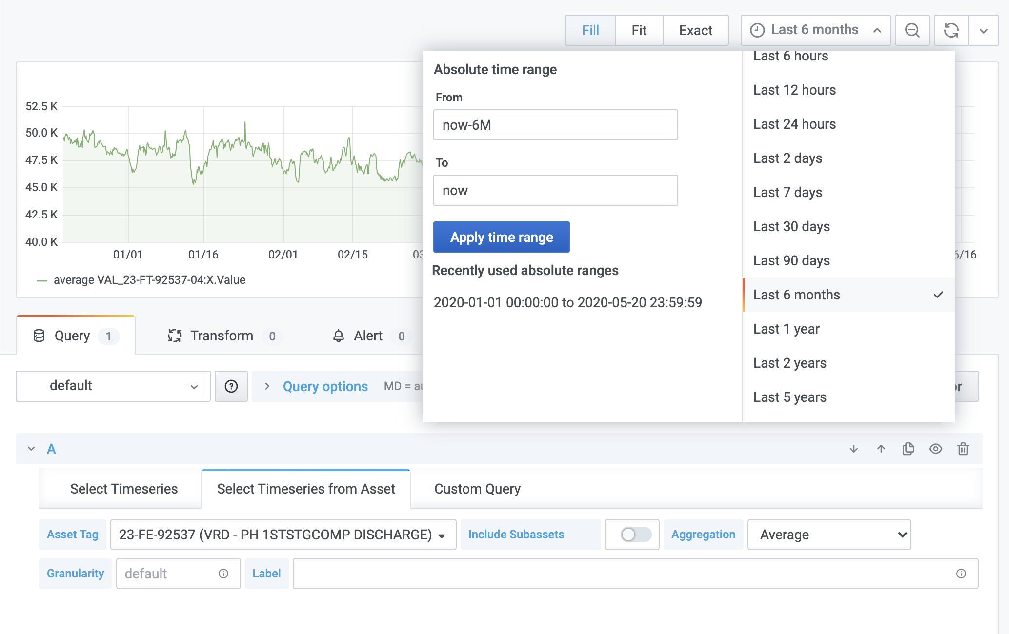
   • Time series search - fetch data from a specific time series. Start typing the name or description of the time series and select it from the dropdown list.

     You can also specify the aggregation and granularity for the query. By default, the aggregation is average, and the granularity is calculated from the time interval selected for the chart.

     tip

     Optionally, set a custom label and use the format {{property}} to pull data from the time series. You can use all the available time series properties to define a label, for example, {{name}} - {{description}} or {{metadata.key1}}.

   • Time series from asset - fetch data from time series related to a specific asset. Start typing the name or description of the asset and select it from the dropdown list. Optionally, decide whether you want to include time series from sub-assets.

   • Time series custom query - fetch time series that matches a query.

3. The time series matching your selection is rendered in the chart area. If necessary, adjust the time to show the relevant data.

   

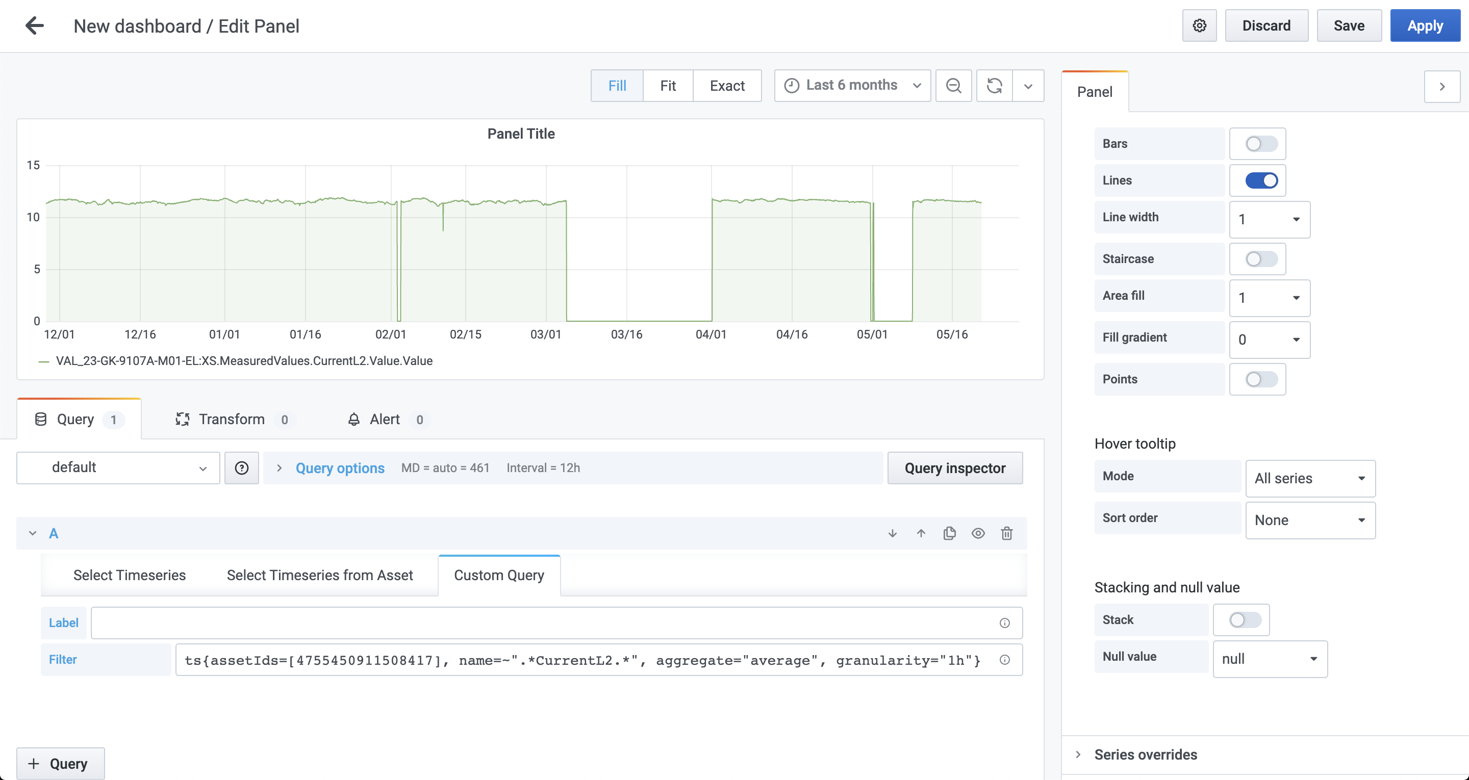
Use custom queries

Use the Time series custom query tab if you want fine-grained control of which time series to fetch. Use a combination of arithmetic operations and functions to define your query and a special syntax to fetch synthetic time series.

Define a query

To request time series, specify a query with the parameters inside. For example, to query for a time series where the id equals 123, specify ts{id=123}.

You can request time series using id, externalId, or time series filters.

For synthetic time series, you can specify several property types:

• bool: ts{isString=true} or ts{isStep=false}
• string or number: ts{id=123} or ts{externalId='external_123'}
• array: ts{assetIds=[123, 456]}
• object: ts{metadata={key1="value1", key2="value2"}}

To create complex synthetic time series, you can combine the types in a single query:

ts{name="test", assetSubtreeIds=[{id=123}, {externalId="external_123"}]}

Filtering

Queries also support filtering based on time series properties which apply as logical AND. For instance, the query below finds time series:

• that belong to an asset with an id that equals 123
• where name starts with "Begin"
• where name doesn't end with "end"
• where name doesn't equal "Begin query"

ts{assetIds=[123], name=~"Begin.*", name!~".*end", name!="Begin query"}

The query contains four types of equality:

• = - strict equality. Specifies parameters for the time series request to CDF. Use with filtering attributes.
• =! - strict inequality. Filters fetched time series by properties that aren't equal to the string. Supports string, numeric, and boolean values.
• =~ – regex equality. Filters the fetched time series by properties that match the regular expression. Supports string values.
• !~ - regex inequality. Filters the fetched time series by properties that don't match the regular expression. Supports string values.

You can also filter on metadata:

ts{externalIdPrefix="test", metadata={key1="value1", key2=~"value2.*"}}

The query above requests for time series where:

• externalIdPrefix equals "test"
• metadata.key1 equals "value1"
• metadata.key2 starts with "value2"

We recommend that you limit the use of regexp filters since they can negatively impact the performance of your dashboard.

This query, for instance, requests all available time series for your project and then filters by names that equal the string some-name:

ts{name=~”some-name”}

Instead, you could replace the regexp with a parameter in the CDF request:

ts{name=”some-name”}

Aggregation, granularity, and alignment

You can specify aggregation and granularity for each time series using the dropdowns in the user interface.

If, for example, the aggregation is set to average and the granularity equals 1h, all queries request datapoints with the selected aggregation and granularity. By default, aggregation with synthetic time series is aligned to Thursday 00:00:00 UTC, 1 January 1970.

With the synthetic time series query syntax, you can define aggregation, granularity, and alignment for each time series separately:

ts{externalId='houston.ro.REMOTE_AI[34]', alignment=1599609600000, aggregate='average', granularity='24h'}

The query above overrides the aggregation and granularity values set in the user interface. See the API documentation for a list of supported aggregates.

Arithmetic operations

You can apply arithmetic operations to combine time series. For example:

ts{id=123} + ts{externalId="test"}

The result of the above query is a single plot where data points are summed values of each time series.

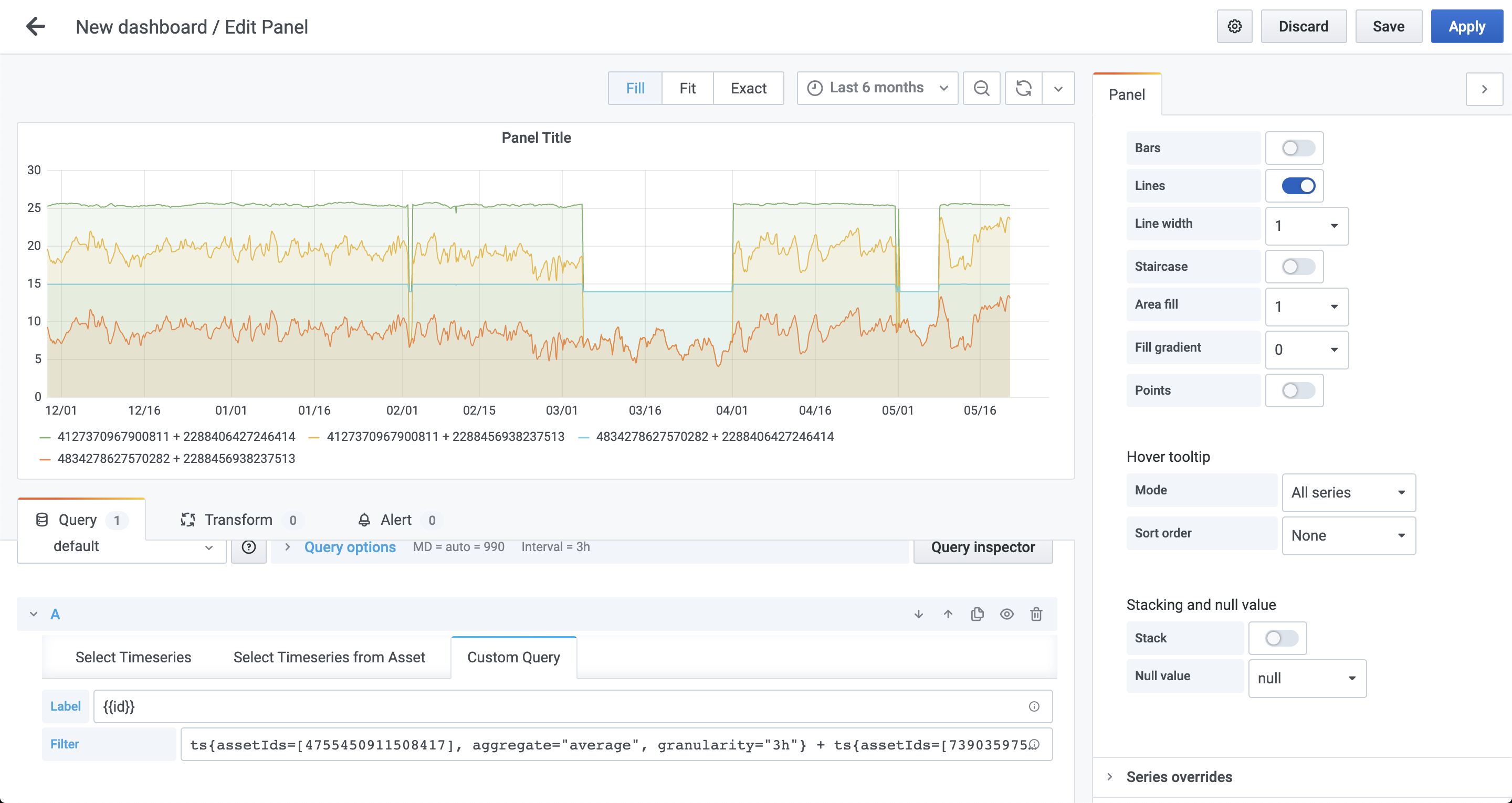
In this example, the query ts{name~="test1.*"} can return more than one time series, but let's assume that it returns three time series with IDs 111, 222, and 333:

ts{name~="test1.*"} + ts{id=123}

The result of the query is three plots, a combination of summed time series values returned by the first and second expressions in the query. The resulting plots represent these queries:

• ts{id=111} + ts{id=123}
• ts{id=222} + ts{id=123}
• ts{id=333} + ts{id=123}

You can see an example of this behavior (each ts{} expression returns two time series) in the image below (notice the labels below the chart).

Functions

We support a wide range of functions that you can apply to synthetic time series:

• Trigonometric: sin(ts{}), cos(ts{}), pi().
• Variable-length functions: max(ts{}, ...), min(ts{}, ...), avg(ts{}, ...).
• Algebraic: ln(ts{}), pow(ts{}, exponent), sqrt(ts{}), exp(ts{}), abs(ts{}).
• Error handling: on_error(ts{}, default_value). See Error handling for calculations.
• String time series: map(expression, [list of strings to map from], [list of values to map to], default_value). See String time series.

Error handling for calculations

The on_error(ts{...}) function allows chart rendering even if some exception appears. It handles errors like:

• BAD_DOMAIN - If bad input ranges are provided. For example, division by zero, or the square root of a negative number.
• OVERFLOW - If the result is more than 10^100 in absolute value.

If any of these are encountered, instead of returning a value for the timestamp, CDF returns an error field with an error message. To avoid these, you can wrap the (sub)expression in the on_error() function:

on_error(1/ts{externalId='canBeZero'}, 0)

String time series

The map() function can handle time series with string values to convert strings to doubles. If, for example, a time series for a valve can have the values "OPEN" or "CLOSED", you can convert it to a number with:

map(TS{externalId='stringstate'}, ['OPEN', 'CLOSED'], [1, 0], -1)

"OPEN" is mapped to 1, "CLOSED" to 0, and everything else to -1.

Aggregates on string time series are currently not supported. All string time series are considered to be stepped time series.

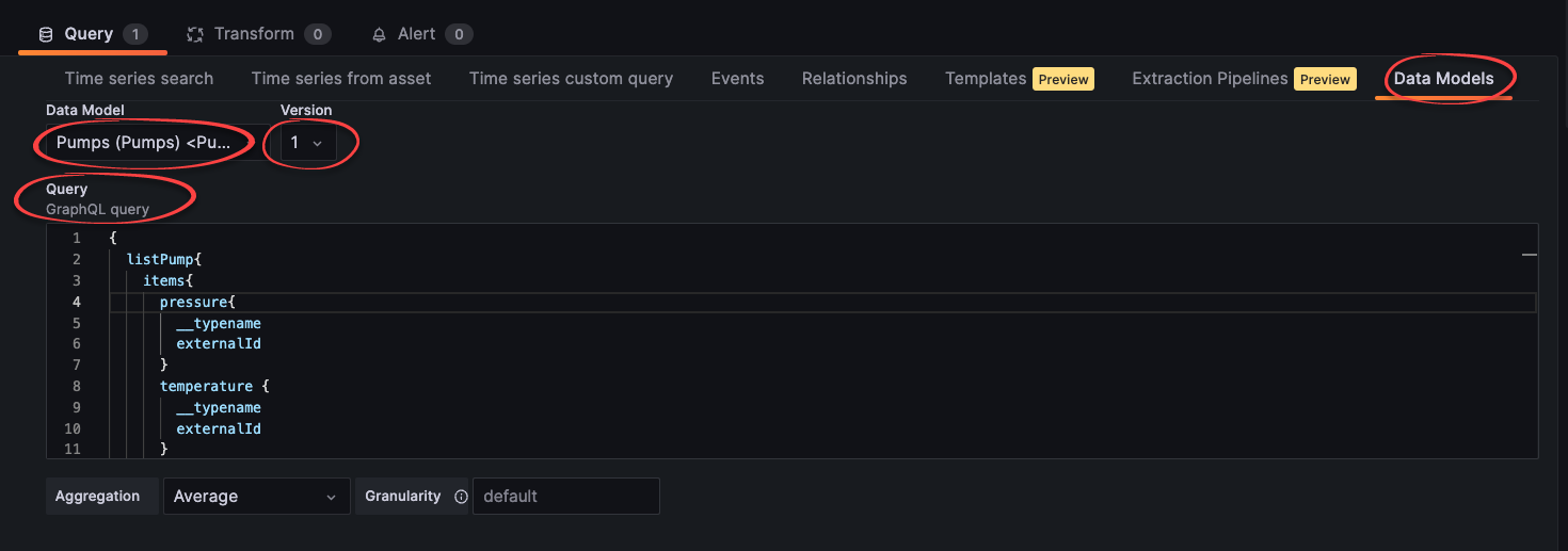
Display time series data from data model instances

You can display time series data from instances of CDF data models:

1. On the Data models tab, select the data model and version.

2. Specify the query.

   important

   Add __typename and externalId below the fields that contain the time series. In this example, below temperature and pressure:

   {
     listPump {
       items {
         temperature {
           __typename
           externalId
         }
         pressure {
           __typename
           externalId
         }
       }
     }
   }